Correction, 23 September 2026. This post says the same call works in water. It does not, and I had not run it in water when I wrote that. Pointed at water the optimiser returns a sane-looking section with a drag coefficient of 0.000000035, which is a hole in the cost function rather than a shape. What that is and what four rounds of fixes did not achieve is in I Said It Works in Water. It Does Not. Everything below about the air case still stands and its numbers are unchanged.
Note, 23 September 2026. The 29 percent saving below is the bottom of the basin the search started in, not the best shape the model allows. Given more evaluations, the same search converges to the same 29.1 percent, so the number stands as reported. Started from a different point, it finds deeper basins, and the model prices one at 46 percent. I do not believe that figure: it belongs to a shape an optimiser found, at a Reynolds number where the transition model, which assumes a perfectly clean surface and calm oncoming flow, is at its most flattering. How that turned up, and what the same search found when asked to delay boiling instead of cutting drag, is in Every Hull Has a Speed Where the Water Boils.
Nine modules in this program carry a drag coefficient. Not one of them could compute one.
Every single figure was typed in from a table of spheres and cylinders. That is honest for a meteorite, which is a rock and will be whatever shape it is. It is useless the moment the question changes from "what does this cost" to "what should this be", which is the only question that matters for a hull, a strut, a fairing, a nose, or water crossing a slope.
So I built the thing that answers it. Same machinery in air and in water, because a shape does not know which it is in: the fluid enters only through the Reynolds number. (That is true of the solver and NOT true of the optimiser on top of it, which is the correction above.)
The method that is exact and gets one number exactly wrong
Outside the very thin layer touching a surface, flow is almost perfectly inviscid, and the equations for that are linear. A panel method solves them cheaply and, for shapes with a known answer, essentially exactly.
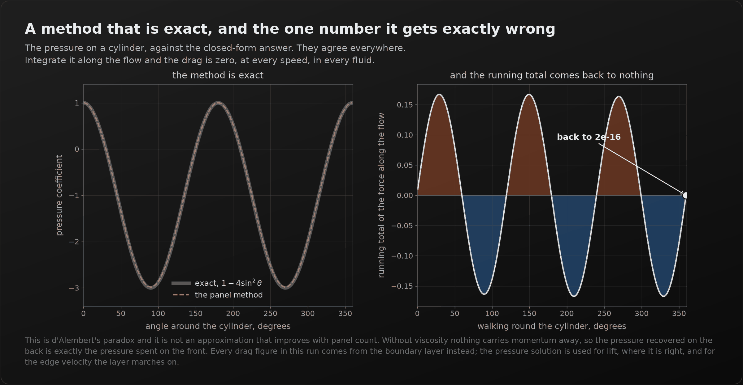
The left panel is the check. The right panel is the problem.
Walk around the body adding up the force along the flow and the total comes back to two parts in ten thousand million million million. That is zero. Not small, not converging toward small: zero, for every closed body, at every speed, in every fluid, at every panel count.
It is d'Alembert's paradox and it is three centuries old. Without viscosity there is nothing to carry momentum away, so the pressure recovered on the back is exactly the pressure spent on the front. I want to be precise about why this is the worst possible failure mode rather than a curiosity: everything around that number is right. The same solve reproduces the exact surface pressure on an ellipse to a tenth of a percent, at any thickness, at any incidence. It gets the lift right. It is fast and it converges. And the one quantity a designer actually wants comes back as a clean, confident, perfectly formed zero.
So every drag figure in this work comes from the boundary layer instead, and the pressure solution is used only for lift and for the edge velocity the layer marches on.
Where it stops
Inside that thin layer, viscosity does everything. Thwaites' method carries the laminar part, Michel's criterion decides where it trips, Head's entrainment method carries the turbulent part, and Squire and Young turn the momentum left in the wake into a drag coefficient. All of that is ordinary, well tested, sixty-year-old engineering, and all of it is checked here against things that are not correlations: Blasius for the flat plate, and Howarth's decelerating flow, where the exact answer for separation is published as 0.120 of the length. Mine separates at 0.1236, which is Thwaites' own published 0.123 rather than Howarth's exact figure. That one percent is the correlation's known error, and the test pins it precisely so it can never quietly be read as agreement.
The important part is where it stops. Once the layer separates, the outer flow I solved is not the outer flow that exists, because the body the fluid now sees is the body plus its wake. The equations do not notice. They will march on past separation and hand back a drag coefficient with four digits on it.
So they refuse instead. Here it is with the refusal in your hands:
That is not a lookup table. It builds a hundred-panel linear system and solves it every time you move a slider, then marches two boundary layers along the surface. Push the incidence up and watch the drag stop being a number rather than becoming a big one. On a phone that can vibrate, you feel it let go.
That is the most useful thing a control on this site does. The refusal is not a value going up. It is a question that stops having an answer.
And I have to be straight about what that refusal is, because it is easy to read as more than it is. Past about eight degrees it gives up, and a real section of that shape flies to about fifteen. What happens in between is that the laminar layer lets go just behind the suction peak, a few percent back from the nose, and then forms a short bubble and reattaches. Reattachment needs the layer's displacement thickness fed back into the outer solution and the two solved together, which is exactly what this does not do. So an early refusal there means the method ran out, not the wing. The widget says so on its own face rather than leaving you to find out.
And then it found the laminar flow aerofoil
The optimiser is the small half: a shape with a handful of knobs, a constraint, and a simplex that turns the knobs.
The constraint is not optional, and this is the refusal I care most about. Minimising drag with nothing else in the statement has an answer, and the answer is a shape of zero thickness, which encloses nothing and is therefore not a body. Ask for that and it refuses, and tells you to say what the thing has to carry.
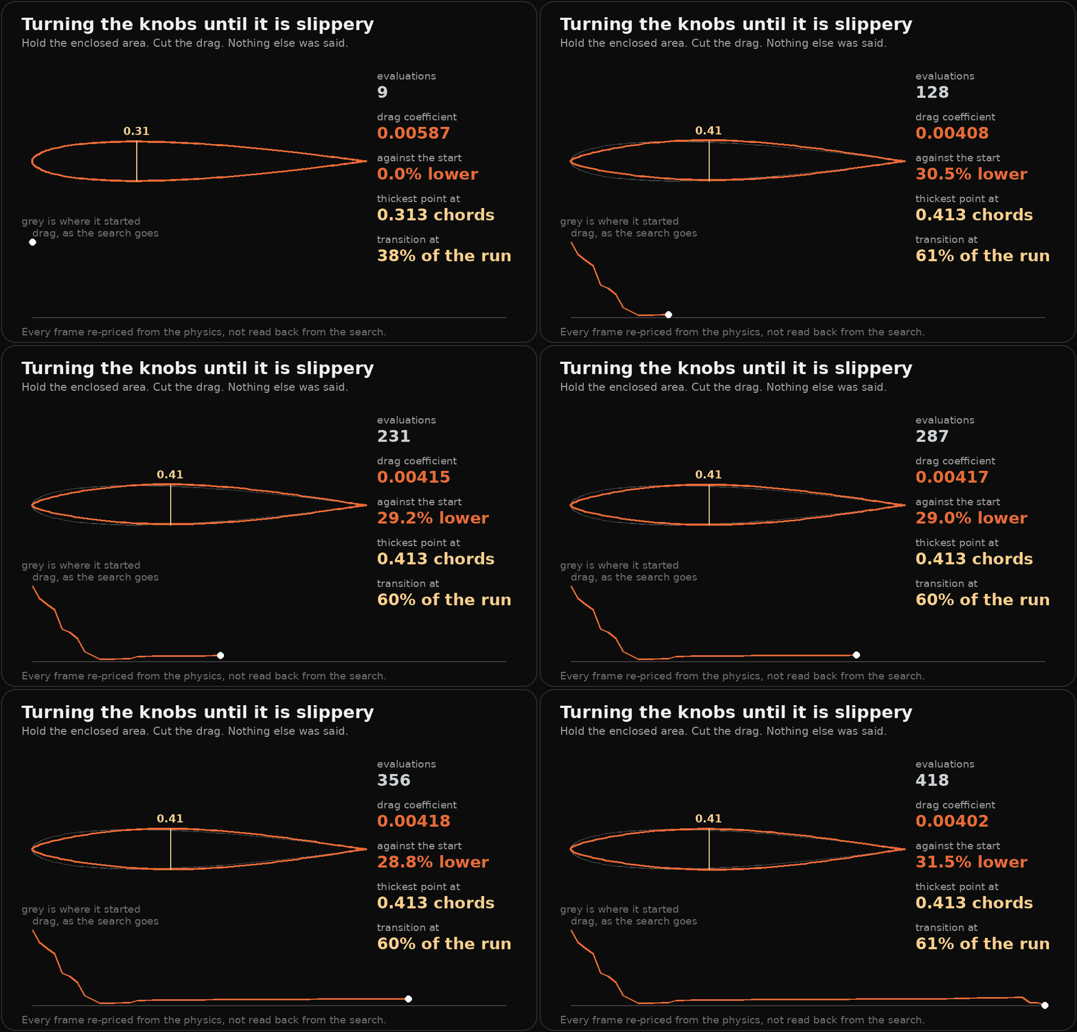
So I told it: hold the enclosed area, keep at least ten percent thickness, cut the drag at three million. Nothing else. No mention of transition, no mention of pressure gradients, no mention of what a good section looks like.
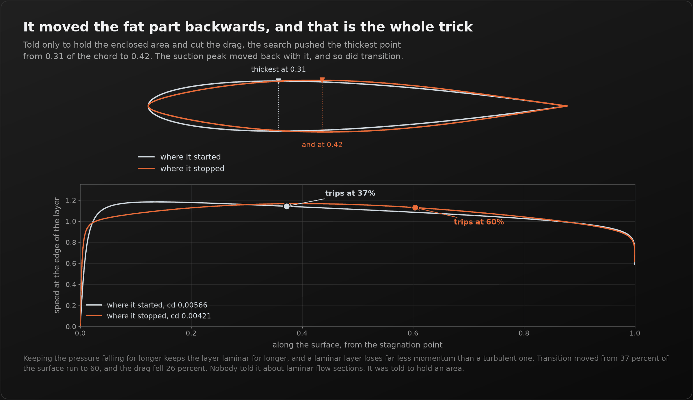
It moved the thickest point from 0.31 of the chord back to 0.42.
That pushed the suction peak aft, which kept the pressure falling for longer, which kept the boundary layer laminar for longer: transition went from 37 percent of the surface run to 60. A laminar layer loses far less momentum than a turbulent one, so the drag fell about a quarter.
That is the laminar flow section. It is what the NACA six-series is, it is why a sailplane wing looks the way it does, and nobody told the search any of it. It was told to hold an area.
Here is the search doing it:
The check that decides whether any of this is real
An optimiser sitting on an approximate method has an obvious way to cheat: find the shape that fools the discretisation rather than the shape that is good. This program has been caught by exactly that before, in a different file, where two grids agreed with each other and both were missing the thing they were measuring.
So both shapes get re-priced at four panel counts. The result is the finding I would keep if I had to throw the rest away:
- the absolute drag coefficient wanders about seven percent across a fourfold refinement, and is not even monotone;
- the saving between the two shapes sits between 26.7 and 28.7 percent at every one of those resolutions.
Both shapes are discretised the same way, so the error is common mode and cancels in the comparison. That is precisely what makes an optimiser legitimate here, because an optimiser only ever compares. It is also exactly why the absolute number must never be quoted to three digits, and why everything above is stated as a fraction saved.
There is a second check underneath it. The module solves this in plain JavaScript; the script that draws these figures solves it again, independently, in numpy, from the equations rather than from the module; and the widget above solves it a third time in your browser. At matched panel count the first two agree to six digits: 0.005310 and 0.003764, a 29.11 percent saving, from both.
The thing I nearly shipped
A panel method needs one more equation than it has surface points, and the usual one is the Kutta condition: the vorticity at the first and last point cancels, so the flow leaves a sharp trailing edge smoothly. That is a real statement about a real edge.
Apply it to a smooth body and it is not a statement about anything, because there is no trailing edge and the "first and last point" is wherever you started numbering. I had it defaulted on. An ellipse at six degrees came back with lift it should not have, a surface speed 142 percent away from the exact answer, and a pressure drag still down at the level of rounding, so nothing in the force integral flagged it at all.
The proof that it was an artefact rather than a result: renumber the same body, starting the point list forty places round, and the invented lift changes. No real force does that.
It is not a default any more. The closure has to be named, and a body with no sharp edge gets told so.
Where this goes
This is one section, in two dimensions, at one incidence, with a transition correlation that carries no roughness and no free-stream turbulence, and it refuses anywhere the flow separates. Those are real limits, and each is written into the module as a named constant rather than living in somebody's memory.
What it already does is the thing I wanted: point it at a body, say what the body has to carry, and get back a shape that is measurably slipperier, with the mechanism visible rather than asserted. The same call works in water. It does not: see the correction at the top. Nothing changes except the Reynolds number, and the Reynolds number is what decides whether the layer trips and where it lets go, which is why the same shape can be fine in one fluid and stalled in the other. There is no single answer to whether a shape is good. There is an answer per fluid and per speed, and the honest version reports both.
The next piece is water on the outside of a body rather than around it: overland flow, where it goes across a slope, and what a swale does with it. Different equations, same discipline. This was the harder half.