Everything I had drawn of this work so far was a number or a curve. I wanted a render: the flow itself, the thing the coefficients are summaries of.
That turns out to be free, and I had not noticed. A panel method solves for a vortex strength on every panel, and once you have those the velocity is computable anywhere, not just on the surface it was solved on. The same influence coefficients that give the surface speed give the field. The only change is that a field point has no panel direction of its own, so setting that angle to zero makes the method's own "tangential" component global x and its "normal" component global y, and the same algebra serves both jobs.
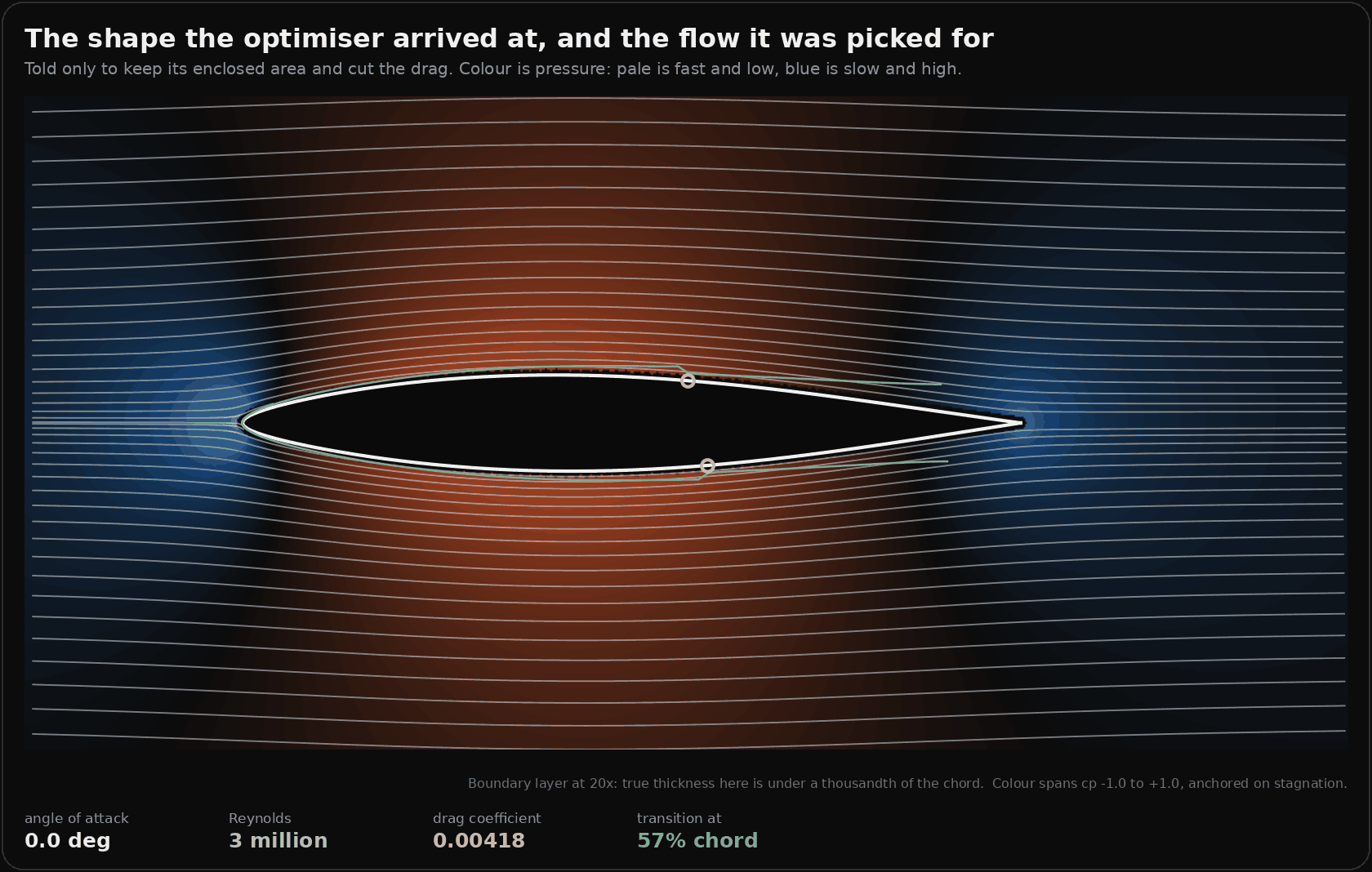
That is the section the optimiser arrived at in the last piece, told nothing except to keep its enclosed area and cut the drag. The warm region is suction, the blue bulbs fore and aft are the flow brought to rest, and the colour scale is anchored on the stagnation point, which is exactly cp = +1 rather than whatever looked good.
The check that lets the picture exist
A streamline plot that is wrong looks exactly like one that is right. There is no visual tell, which is the same problem as every other figure here and worse, because a render is persuasive.
So the field evaluator is checked against the surface solution it came from. Probe just outside each panel and you must get that panel's own surface speed back:
| probe offset | median relative error |
|---|---|
| 0.020 chord | 9.9e-3 |
| 0.005 chord | 2.0e-3 |
| 0.001 chord | 3.0e-4 |
First order convergence, which is what a panel method should give. There is a second check for free: a closed vortex sheet carries no flow inside itself, and probing the middle of the body returns a speed of 1.2e-5. Both run every time the figure is generated and both print.
Finding the outward normal was done the same way rather than by reading the code. The panel normal the force sum uses points inward for this point ordering, and a probe offset along it lands inside the body, where the answer is correctly almost zero. A render built on that sign shows a body sitting in still air.
Then I pointed it at both shapes
The plan was to turn the body until its boundary layer let go, because the refusal is the interesting frame. What came out was better than the plan.
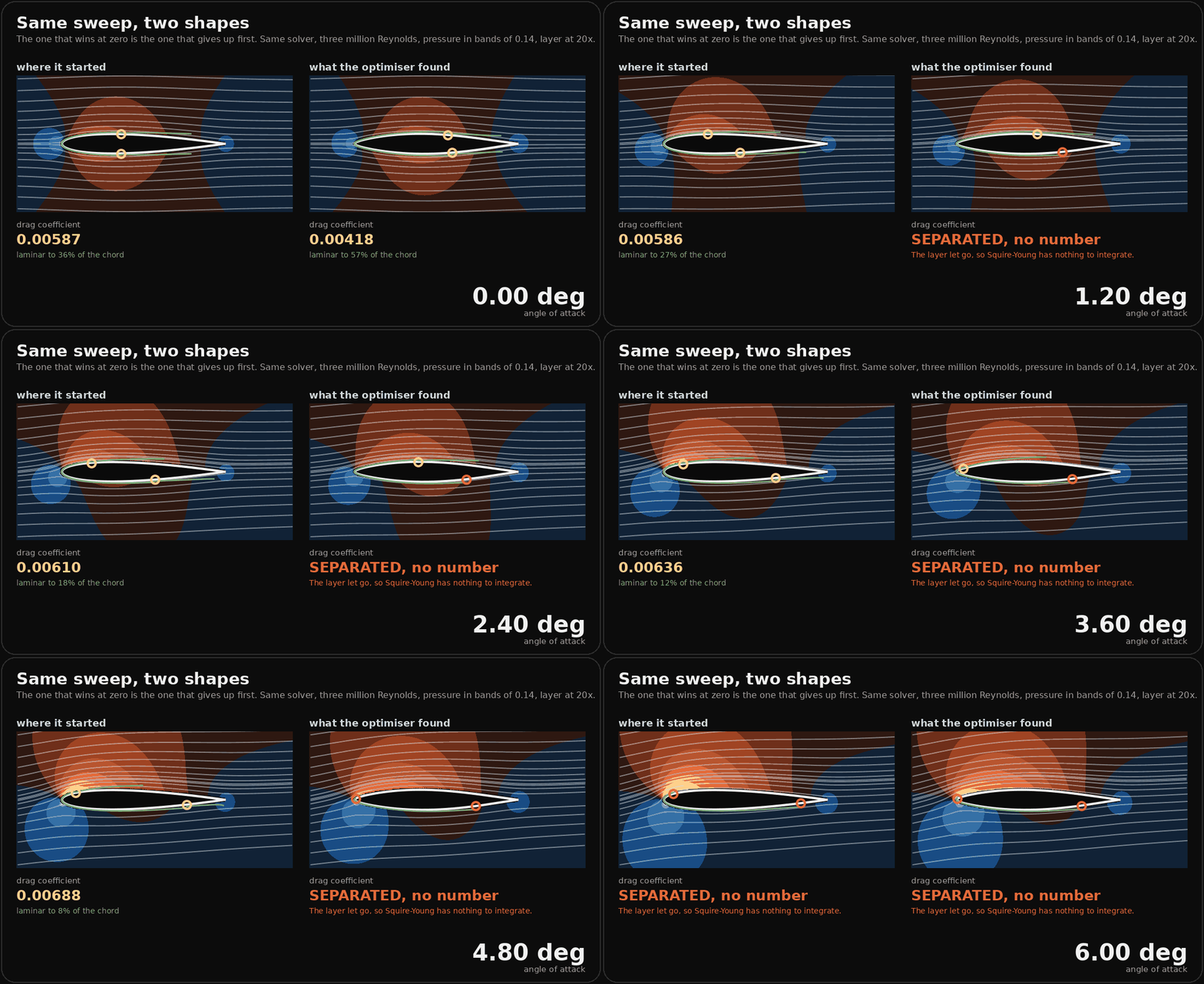
At zero incidence the optimised section is better by every measure I had asked for. It carries 29 percent less drag and holds a laminar boundary layer over 57 percent of its surface against 36 percent.
It gives up under a degree. The section it started from holds to nearly six.
Before that becomes a claim, it has to survive the same test the drag saving had to survive, and it half does. Re-priced at 120, 160, 240, 320 and 400 panels:
| panels | started with | optimised |
|---|---|---|
| 120 | 5.50 deg | 0.25 deg |
| 160 | 5.75 deg | 0.00 deg |
| 240 | 5.75 deg | 0.75 deg |
| 320 | 5.75 deg | 0.25 deg |
| 400 | 5.50 deg | 0.75 deg |
The starting section is resolved: 5.50 to 5.75 degrees across a fourfold refinement. The optimised one is not. It wanders from zero to three quarters of a degree, a spread wider than its own value, which means this method at these resolutions cannot tell you what its usable range is, only that it is small. So the number in the animation is not a measurement and I am not quoting one. What survives refinement is the comparison, which is stark at every resolution: one of these holds about 5.6 degrees and the other holds under one.
There is a second caveat and it cuts the same way. This solver has no separation bubble model, so a laminar separation that would reattach in reality is reported as a refusal rather than as a bubble. A real laminar flow section does have a usable bucket a couple of degrees wide. The honest reading is that the refusal angle is a floor rather than an estimate, and that the direction of the finding, not its size, is what I am standing behind.
That direction is not a bug in the optimiser and it is not a bug in the solver. The optimiser minimised drag at one angle of attack, subject to holding an area, and it found a shape that is superb at that angle and has almost no usable range around it. The long favourable pressure gradient that keeps the layer laminar for 57 percent of the chord is the same gradient that has to be paid back over a shorter distance aft, and a laminar layer asked to climb a steeper hill lets go sooner.
This is the well known trade on laminar flow sections and I did not put it in. It fell out of the same machinery, asked a question the optimiser was never asked.
The part that should make anyone nervous
There is no line anywhere in the optimiser's output that says this. It reports a drag coefficient, a saving, a thickness and where the thickest point moved to. Every one of those numbers is correct. Nothing is flagged, because nothing asked, and an objective function has no way to tell you what you left out of it.
The result is a well formed answer that is true about the question asked and false about the question meant, which is the same shape as everything else on this blog: the confident number, in the right units, that nobody has a reason to doubt.
The honest version of the earlier result is therefore two sentences rather than one. Told to hold an area and cut the drag, the optimiser rediscovered the laminar flow section. Told only that, it also discovered why nobody builds an aircraft out of one without thinking hard about the rest of the flight.
And I made the module's own mistake while drawing it
The first version of these renders asked for the smooth closure on every solve.
These sections have a sharp trailing edge, so the Kutta condition is a statement about a real edge and is the correct choice. Smooth is not. Nothing errored, nothing looked odd, and every picture came out.
It was caught by the cross-check at the bottom of the script, which re-prices both sections and requires the module's published pair back. At 120 panels, from the script: 0.005310 and 0.003764, a saving of 29.11 percent. From the module: 0.005310 and 0.003764, a saving of 29.11 percent. With the wrong closure the same line read 0.004101 where the module said 0.004181. Two percent, which is comfortably inside what anyone would read as rounding, and it was the only thing on screen that knew.
I should be precise about what that error did and did not do, because my first draft of this paragraph overstated it. It did not move the separation angle: both closures hold to 0.75 degrees at 240 panels. All it did was return a quietly wrong coefficient, which is the more dangerous of the two outcomes, since a picture that falls over is a picture you fix.
That is the last piece's headline finding arriving from the other direction. There I had the Kutta condition defaulted on where it did not belong and it invented lift outright. Here I had it defaulted off where it did belong and it shaved two percent off a drag coefficient. The module made me name the closure; the figure script had a default; the default was wrong.
Two notes on the drawing
The boundary layer is drawn at twenty times its real thickness and the caption says so, in the picture. At three million Reynolds the displacement thickness on this body is under a thousandth of the chord, which is a third of a pixel. Drawn true it is invisible, and the render then implies the body is dry. Drawn exaggerated without the label it implies the layer is centimetres thick. The multiplier belongs next to the thing it multiplies.
It also has to be capped. Approaching the trailing edge the shape factor climbs, so twenty times a rising thickness leaves the body and shoots off the frame as two green horns. That is the exaggeration failing rather than the layer doing anything, so the curve stops where the cap bites.
The neutral colour has to sit exactly on zero pressure. My first map ran from cp = -1.1 to +1.0, so undisturbed air landed at 0.52 of the ramp, which was brown, and the entire far field rendered as a warm haze. The picture claimed a disturbance reaching the edge of the frame. Autoscaling to the visible field is worse and I tried that too: the window is mostly far field where cp is a few hundredths, so the span collapsed and still air two chords out came back saturated blue.
A physical anchor beats a statistical one. Incompressible flow brought to rest has cp = 1 wherever it happens, so the scale runs from -1 to +1 and background is background.
Have a go
Six bodies, the same solver, running in your browser rather than replaying anything. The streamlines are traced through the real velocity field, the drag is computed from the same equations as every figure above, and the incidence slider will take each of them past the point where the answer stops existing.
Worth trying: put the teardrop and the fat strut side by side at zero and then walk the incidence up. The teardrop is far slipperier and quits almost immediately. The strut is draggy and keeps answering. That is the whole finding above, in a control you can feel.
The fluid slider is the other one worth moving. Nothing about the shape changes when you switch from air to water, because a shape does not know which it is in: the fluid enters only through the Reynolds number, and what the Reynolds number decides is where the boundary layer trips and whether it holds on.
One caveat that is not a detail. Every body here is a section, which means it is two dimensional and infinite in the third direction. A real hull has ends, a real wing has a span and a tip, and both have a wake this method does not model. None of these numbers is a drag figure for an actual craft. What they compare honestly is each other, in the same fluid, at the same angle.