The last piece I built made a shape slippery. This one is the other half I said was harder, and it was, though not for the reason I expected. The equations are easier. The lying is subtler.
Water crossing ground is two questions stacked. How much soaks in, and where does the rest go. The first is Green and Ampt, which is a sharp little piece of physics: a wetting front advances into the soil, the suction at that front pulls water in faster than gravity alone would, and the rate decays as the column above the front gets longer. The second is Manning and the kinematic wave, which routes what is left down the slope.
Both are textbook. Both are in the module. Neither one is the finding.
The check that never fires
There is a standard way to decide whether the kinematic wave is allowed. Woolhiser and Liggett give a dimensionless number, k, and the rule is that the kinematic approximation is good above about 10 and questionable below it. I wrote it in, wrote a test that fed it dead flat ground, and expected a refusal.
It came back with k = 325.
The number is k = S₀L / (h₀Fr²), and if you substitute the Froude number back in, it reduces to gS₀L / v₀². The velocity is squared in the denominator. Sheet flow on turf moves at centimetres a second, so the Froude number is hundredths and k is enormous everywhere. Worse than enormous: flatter ground makes the flow slower, which makes k larger. The check gets more confident exactly as the ground gets flatter, which is the opposite of the warning it was meant to give.
A check that never fires is worse than no check, because it sits in the output looking like due diligence. So the number is still computed and still returned, so a reader can see it is meaninglessly large, and the actual refusal is somewhere else entirely.
What actually decides it
The refusal that works is not a dimensionless group. It is a comparison of two lengths.
A plane is the right model when the fall along the flow path is large compared with the bumps in the surface. Graded soil under established turf is flat to somewhere between one and three centimetres. So a thirty metre run at one in fifty falls 600 mm, which is twenty times the bumps, and a plane is fine. The same run at one in two thousand falls 15 mm, which is half the bumps, and there is no plane there at all. The water does not run down that slope. It sits in the dips and leaves along whatever line happens to join them, which is a property of the surface and not of the gradient.
That is the module's refusal, and it says so in those terms rather than returning a number:
This slope falls 15 mm over its 30 m, against ground that is flat to about 30 mm. The fall needs to be several times the bumps before a plane is the right idea, and here it is 0.5 times.
You can walk it into that state yourself. The slider below solves the whole chain live, Green-Ampt and all, and refuses when the fall stops being a fall.
Three things in there are worth pulling out.
Manning's n for vegetation is a depth, not an uncertainty band. Every table gives dense turf as something like 0.04 to 0.40, and it reads exactly like a range you would take the middle of. It is not a range. It is a curve: at one millimetre the water is moving through the grass and n is 0.40, at a hundred millimetres it is moving over the grass and n is 0.04. Taking 0.22 as a constant is wrong by a factor rather than by a percentage, and at the depths sheet flow actually reaches it is wrong in the direction that makes the water arrive too fast.
Every soil number is transcribed and every one defaults to its unfavourable end, which here means the slowest conductivity and the least pore space, because that is the end that makes more runoff. A design that works at the pessimistic end works. A design that only works at the friendly end depends on a number nobody measured on that site.
There is no default storm. The module refuses to have one. An intensity is regional, it comes from a published depth-duration-frequency source for the actual place, and a built-in value would be the single largest assumption in the answer wearing the clothes of a constant.
The thing the plane model cannot do
Here is the part that made the second module necessary.
The kinematic wave drives flow with the bed slope. That is what makes it a closed form, and it is why it is in every tool. It also means that on flat ground, the driving term is zero, and the water does not move. Not slowly. At all. And yet the depth it reports is perfectly finite, the arrival time is perfectly finite, and nothing in the output says the answer describes water that is standing still.
A model that cannot make a puddle will still tell you how deep the water is. It is the same shape as everything else on this blog: a well formed answer, in the right units, with the right sign, that happens to be false.
The fix is to drive the flow with the water surface slope instead of the bed slope. That is the diffusive wave, it costs the closed form, and it buys the one behaviour that matters: water can pile up until its own surface is tilted, and then it moves. A hollow fills until it is level and then spills. That is the whole difference, and it is what a plane could never do.
So the second module is a two-dimensional march over a real surface. Four neighbours, explicit, first order, with the flux between any two cells set by the slope of the water on top of them.
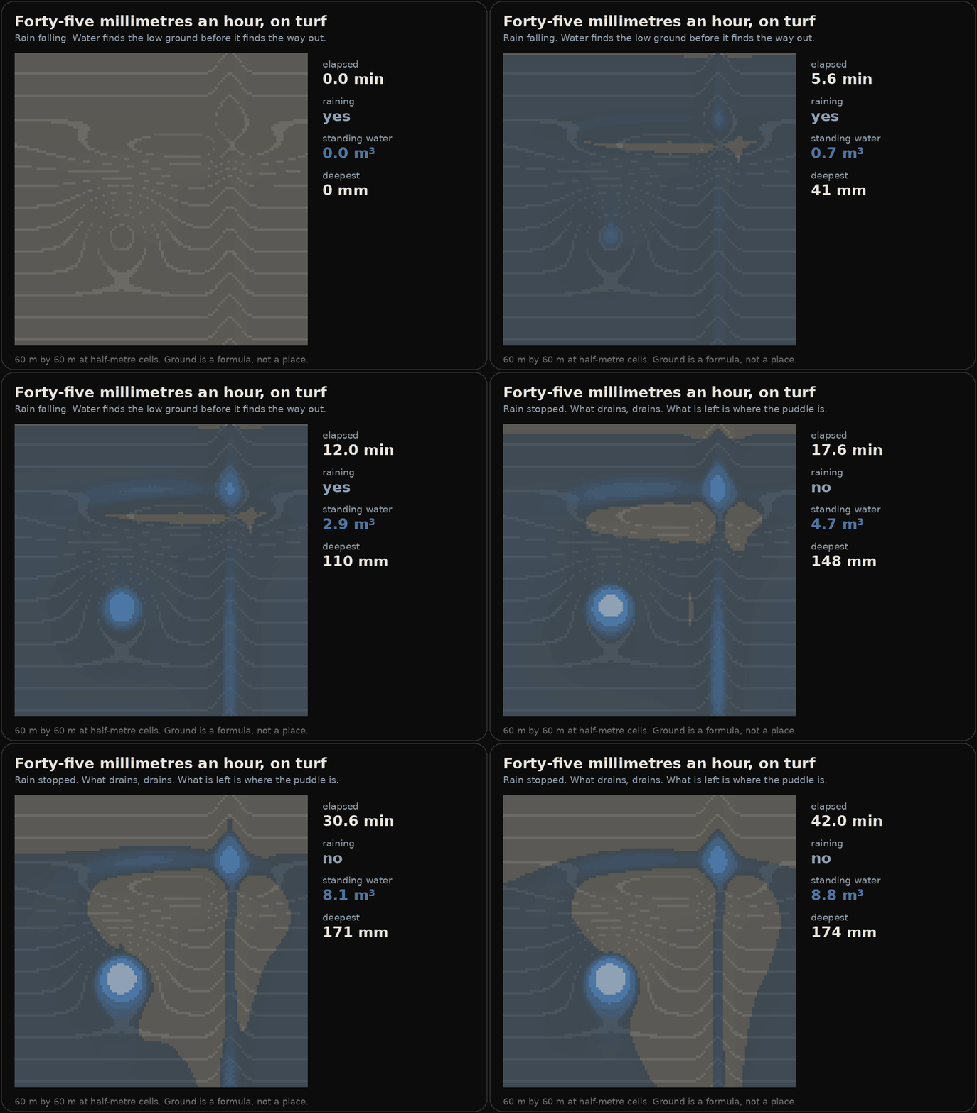
Sixty metres by sixty, at half-metre cells. The ground is a formula rather than a place: a constant fall, one hollow, one ridge across the fall, one shallow cut. Forty-five millimetres an hour for sixteen minutes, then twenty-six minutes of drainage.
Nothing in that run was told where the low ground is. Rain fell everywhere at the same rate. The two pools are where they are because the solver found them.
Mass balance, and the three attempts it took
A flood model that loses water produces a beautiful picture and there is no way to see the loss by looking at it. So the only check that matters is arithmetic: rain in, minus what left the domain, minus what is still on the ground, equals zero.
It does, to zero exactly on the drainage run and to 9e-11 on the rainfall run. Getting there took three goes at one piece of the solver, and the failures are instructive because every single one of them conserved mass perfectly while being wrong.
The problem is that an explicit scheme can take more water out of a cell in one step than the cell has. Left alone that makes the depth negative, and a negative depth gets clamped to zero somewhere downstream, and that clamp is water created out of nothing. So you need a limiter.
First attempt: cap each face at half the drop between the pair. That is the right idea for two cells in isolation. A cell has four faces, and if all four are draining, the cap fires four times and empties the cell completely in one step. The bowl held a cone that never spread, with the centre alternating between 0.122 and 0.244 every step. The average of those two was exactly the right answer. Mass was conserved to eleven figures throughout.
Second attempt: cap each cell at half the water it holds. Better, still a two-cycle.
Third attempt, which works: a cell feeding n neighbours is sharing a drop with each of them, so its fair share of any one drop is one part in n+1, and the most it may give away in total is the sum of its drops times the area over n+1. That converges monotonically: 0.18253, 0.18280, 0.18288, 0.18292, against a bisection on the geometry that says 0.18296.
Then there was a fourth, which was not the limiter at all. Water leaving the edge of the domain was not being counted as one of those faces, so the outlet cells were rationed against a share that ignored the only direction they could actually drain. A plane that should have shed to four millimetres flooded to 285. The mass balance was exact the entire time, because the water was conserved into the wrong place, which is precisely the failure mode a conservation check cannot see. That is the same lesson this program keeps relearning: a conserved quantity is not a second route. The wrong orbit can be conserved perfectly.
Where it ended up
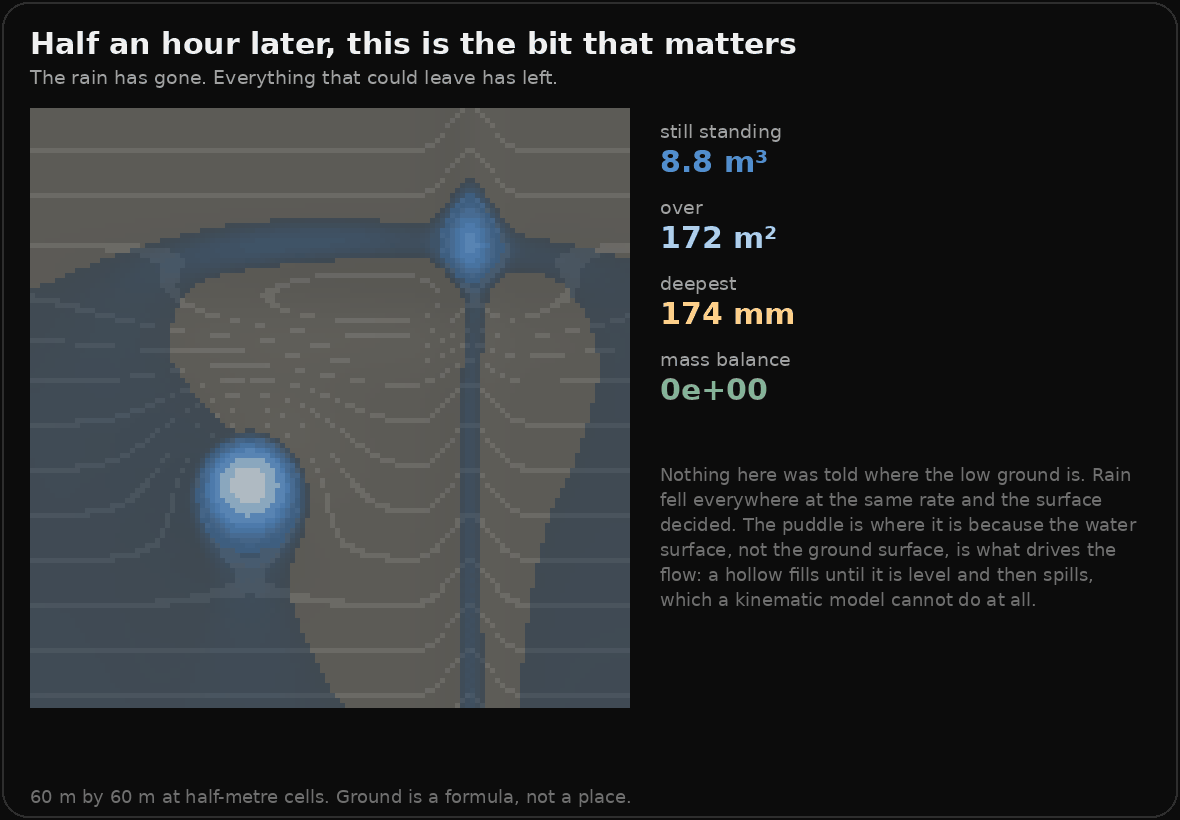
Forty-three point two cubic metres of rain fell, which is arithmetic rather than a result. Twenty point seven are still on the ground when the run ends and twenty-two point five have left the domain, and those two account for every drop. Eight point eight cubic metres are standing, over a hundred and seventy-two square metres, a hundred and seventy-four millimetres at the deepest point.
Standing means something specific and chosen: at least five millimetres deep, with no neighbour whose water surface is lower by more than a millimetre. Both of those are choices and both are written into the module as named constants rather than buried inside a comparison. The tolerance is there because a settled pool is not exactly level, it is level to a fraction of a millimetre, and requiring strictly no lower neighbour found only the few cells at the very bottom and reported a fifth of a puddle.
The two implementations, and why the pin exists
Everything on this site is drawn by a script that solves the problem again, independently, in numpy, from the equations rather than from the module. That is the standing rule here, and it is worth exactly nothing if nobody ever compares the two.
So the ground is a closed form written identically on both sides, and the engine's test suite builds the same surface and asserts the figures above. The two repositories cannot import each other, so the pin is the only thing joining them.
It earned itself immediately. The figure script drained one edge of the domain, on the reasoning that the ground falls that way; the module drains any edge cell whose inward neighbour is higher, and on a surface with a hollow and a cut in it that is not the same set. The two disagreed by five percent on the integrals while the deepest point agreed to half a percent.
That ratio is the tell. A solver difference moves everything. A boundary difference moves the totals and leaves the interior alone, and knowing which one you are looking at is the difference between an afternoon and a week. They now agree to about a part in ten thousand on the volumes; the standing-water figure still differs by about one percent, because that is a per-cell classification against a threshold and a hair of depth moves a cell in or out at a puddle's edge. The test's tolerance says so explicitly, rather than being tightened until it only passes by luck.
What it still cannot do
Pits are not filled. A real grading tool pre-processes the surface to remove depressions that are artefacts of the survey, because it needs every cell to drain somewhere. This one does not, and the reason is that here a depression is usually the answer rather than the artefact. Filling them would remove the thing being looked for.
The cell size hides whatever is smaller than the cell size, and it travels with every answer rather than sitting in a header. Half-metre cells cannot see a wheel rut, and a wheel rut is a drainage path.
And the ground in every figure here is a formula. Give it a real surface and the arithmetic is the same; the honesty of the answer then depends entirely on the survey, which is somebody else's instrument and somebody else's error bar.
None of which changes the part I actually wanted. Point it at a piece of ground, rain on it, and watch where the water decides to be. Nothing tells it where the low spot is. It finds it, and then it tells you how much is sitting there and how long it took to arrive, and when the model has no business answering at all, it says that instead.
Dig your own
The animation above ran on ground I wrote as a formula. Here is the same solver on ground you shape.
This one is not a re-implementation. Every other control on this site solves its physics a second or third time on purpose, so the module, the figure script and your browser are independent routes to the same answer. That works when the physics is a closed form two hundred lines long. It does not work here: the outflow limiter in this solver took three attempts, and two of the wrong versions conserved mass to eleven figures while oscillating. A hand copy would have been a fourth thing nobody checks.
So the file your browser is running is the engine's own, copied across, and a check in this repository holds the copy to the figures printed above: 43.2 cubic metres of rain, 20.696 still on the ground, 22.504 gone, mass balance zero. If the copy drifts, those numbers move and the check fails.
Which is why the mass balance is on screen while you play. It is the only readout that tells you whether the picture is arithmetic or decoration, and it should sit at zero the whole time, including while you are digging.
Two things worth trying. Dig a hollow partway down the slope and watch it fill and then spill, which is the behaviour the kinematic wave cannot produce at all. And drag the fall slider to flat: the water stops going anywhere in particular and starts sitting wherever you dug, which is exactly the regime where the one-dimensional model earlier in this post refuses to answer.